TL;DR

• Propensity models predict payment likelihood before default occurs
• Default propensity and payment propensity are two distinct model outputs
• Behavioural signals outperform static credit attributes in collections
• Explainability is non-negotiable under SR 11-7 and ECOA
• Survivorship bias and target leakage are the two most common build failures

Once an account transitions to default, the probability of curing it drops to 7%.

That single figure, drawn from research on consumer credit default transitions, is the entire business case for propensity modelling in collections. The probability of a current account transitioning to default sits at 23%. The probability of recovering an account that has already defaulted sits at 7%. The math is unambiguous: intervening before default is roughly three times more likely to produce a positive outcome than recovering after one.

Yet most US bank collections teams still build their operational workflows around days-past-due buckets. They react to a missed payment, assign the account to a queue, and begin the recovery process. The DPD model is a lagging indicator. It tells you what already happened. A propensity model tells you what is about to happen, and it gives you time to intervene before the cost of doing so multiplies.

This article is a practical guide to what collections propensity models actually predict, which signals make them work, how to build and validate them to SR 11-7 and ECOA standards, and how to turn a propensity score into a contact strategy that recovers more at lower cost.

What a Collections Propensity Model Actually Predicts

The term “propensity model” covers two distinct predictions in a collections context, and treating them as interchangeable is a common and expensive error.

Default propensity predicts the probability that a currently performing account will miss a payment in the next 30, 60, or 90 days. This is the early warning signal. It applies to accounts that have not yet entered the collections workflow and enables pre-delinquency interventions: proactive payment reminders, hardship plan offers, and pre-emptive contact before an account becomes a collections case. The INFORMS research on propensity to pay models describes this as predicting “whether the customer will pay on time, before 30 days or 60 days from the due date,” with the model applied at various intervals in the account lifecycle.

Payment propensity predicts the probability that an account already in delinquency will make a voluntary payment in the next 30 days, given the current state of the account and the available contact and treatment options. This is the collections strategy signal. It does not ask whether an account will eventually pay. It asks which delinquent accounts, if contacted today through which channel and with which message, are most likely to self-cure before the cost of the recovery process escalates.

It is also worth distinguishing both from a churn prediction model. A churn prediction model forecasts whether a customer will voluntarily disengage from a product or service, closing an account or switching providers. A collections propensity model targets an involuntary behaviour: payment failure driven by financial stress. The signal sets, intervention timing, and regulatory validation requirements are fundamentally different for each.

Both models matter. But they operate at different points in the delinquency lifecycle, they use different feature sets, and they require different validation approaches. Most banks that deploy only one are leaving significant recovery opportunity on the table. The business logic is clear: default propensity captures accounts before they cost money to recover; payment propensity optimises how that recovery cost is allocated once delinquency has occurred.

The Input Signals That Actually Matter

A credit scorecard and a collections propensity model share a superficial resemblance. Both ingest customer data. Both produce a risk score. The critical difference is in the signals they prioritise.

A credit scorecard is built on relatively static credit bureau attributes: payment history, utilisation, age of accounts, inquiries. These attributes change slowly. They are well-suited to underwriting decisions made at a single point in time. Traditional credit risk scoring frameworks rely on precisely these stable, point-in-time signals, which is why they fall short when applied to the dynamic, week-to-week behavioural patterns that determine collections outcomes.

A collections propensity model needs signals that reflect current and changing behaviour. The accounts it scores are people whose financial circumstances are shifting, whose engagement with their bank is a real-time indicator of intent, and whose payment likelihood can change week to week.

Four categories of signals consistently outperform traditional credit attributes in collections propensity contexts.

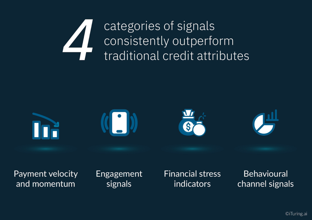
Payment velocity and momentum. How the pattern of payments has changed in the last 30 to 90 days, not just whether a payment was missed. An account that has progressively reduced payment amounts across three consecutive cycles is a different risk profile from an account that missed a single payment after years of consistent full payment. The trajectory matters as much as the current state.

Engagement signals. Whether the customer has logged into their account recently, opened payment communications, initiated contact with the bank, or clicked through to payment options in digital channels. Research on intelligent collections strategy consistently identifies customer-initiated engagement as one of the strongest predictors of voluntary payment. A delinquent customer who opened a payment reminder email yesterday is fundamentally different from one who has not engaged with any communication in 45 days.

Financial stress indicators. Patterns across the customer’s broader relationship with the institution that indicate stress: declining balances across accounts, increasing utilisation on revolving credit, missed payments on multiple products simultaneously, or recent overdraft activity. These cross-product signals often appear two to four weeks before a collections-stage missed payment.

Behavioural channel signals. Which contact channels the customer has responded to historically, at what times of day, and with what outcomes. A customer who has never responded to a voice call but has a 40 percent email response rate requires a fundamentally different contact approach from one with the inverse pattern.

Model Architecture: Why Explainability Is Non-Negotiable

The collections propensity model architecture question often gets framed as a performance versus interpretability trade-off. It is not quite that simple.

Gradient boosting models, including implementations like XGBoost and LightGBM, consistently perform well in collections propensity contexts. Research specifically on LightGBM in financial services propensity modelling demonstrates strong performance on both accuracy and computational efficiency for large collections portfolios. They handle mixed feature types, manage missing data gracefully, and produce well-calibrated probability outputs that map cleanly to propensity score bands.

Neural network architectures can outperform gradient boosting on raw predictive accuracy, particularly when engagement signal data is rich and high-dimensional. The ArXiv deep learning research on consumer default prediction shows consistent improvements over traditional scoring models. The tradeoff is interpretability: neural networks produce predictions that are substantially harder to explain at the individual account level.

For US bank collections AI, that interpretability gap is a compliance problem, not just a technical preference.

SR 11-7 requires that model logic “can be reasonably understood by qualified individuals,” and explicitly requires conceptual soundness validation and ongoing monitoring of model behaviour. ECOA requires that adverse action notices provide specific reasons for credit-related decisions. Shapley values (SHAP) provide the individual-level explanations needed to satisfy ECOA adverse action requirements, and they are now the standard approach for demonstrating explainability in OCC and Federal Reserve model examinations.

A collections propensity model that cannot produce account-level SHAP explanations is a regulatory liability, regardless of how accurately it predicts. The practical solution for most US banks is a gradient boosting architecture with built-in SHAP explainability, rather than a neural network that requires post-hoc approximation to satisfy examination requirements.

Model Risk Management and Validation Requirements for Collections Propensity Models

Model risk management for collections propensity models under SR 11-7 requires four specific validation components, each of which addresses a different potential failure mode.

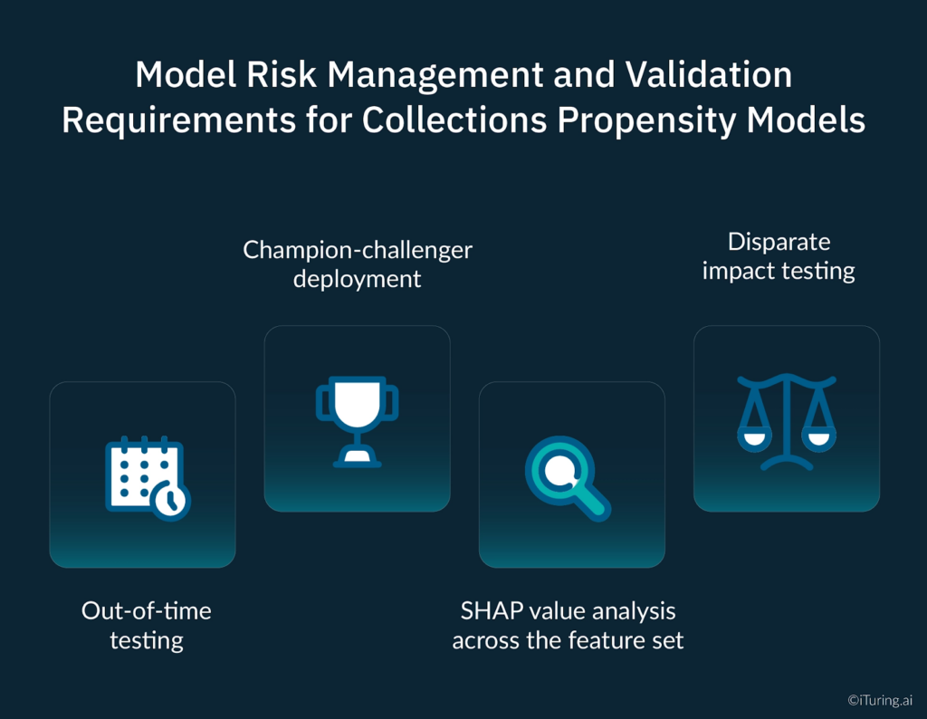
Out-of-time testing. Standard cross-validation splits training and test data randomly. Out-of-time testing splits them chronologically, holding out the most recent time period as the test set. This matters for collections models because payment behaviour patterns shift with economic conditions. A model that validates well on random splits but performs poorly on out-of-time data is overfitted to a historical period that may no longer reflect current conditions. For OCC examination purposes, out-of-time test results are a core component of the conceptual soundness validation.

Champion-challenger deployment. After initial validation, routing a defined proportion of production accounts through a challenger version alongside the production model, a champion challenger model structure, provides continuous empirical evidence of performance under live conditions. This is particularly important for self-updating architectures, where the version examined during initial validation may differ meaningfully from the version running three months later. SR 11-7 specifically contemplates ongoing performance benchmarking against alternative estimates as part of the ongoing monitoring requirement.

SHAP value analysis across the feature set. Validating that the features driving predictions are conceptually sound, legally permissible under ECOA, and stable across demographic segments. A model that assigns high predictive weight to a feature correlated with protected class membership requires scrutiny regardless of whether that feature is itself a protected attribute. SHAP analysis surfaces these correlations at the feature importance level, allowing the model risk team to evaluate them before deployment rather than after an adverse finding.

Disparate impact testing. Running the model’s output score distributions and downstream contact strategy decisions across protected classes to test for differential treatment outcomes. Under ECOA, a disparate impact finding can arise from a facially neutral model if its practical effect is disproportionate treatment of protected groups. This testing must be documented, submitted as part of the validation package, and repeated at each revalidation cycle.

Translating Propensity Scores Into Collections Strategy

A propensity model produces a score. That score needs to drive a decision. The decision is which account gets which contact treatment, through which channel, at what intensity, and with what message. Getting this translation right is where the ROI from propensity modelling is actually realised.

The standard approach is score banding: dividing the score distribution into segments that receive differentiated treatment. Three to five bands typically cover the range of meaningful treatment variation.

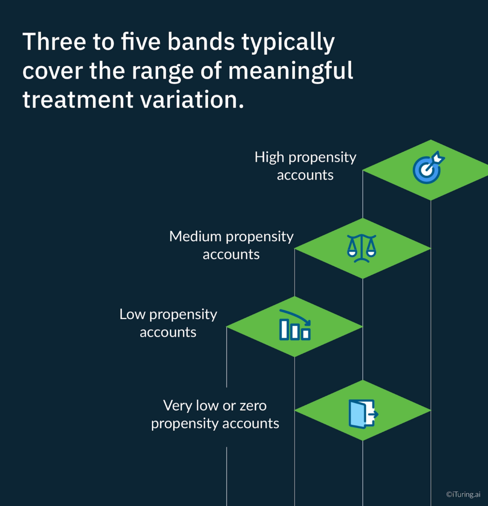
High propensity accounts are accounts with a strong probability of voluntary payment given appropriate contact. These accounts need timely, low-friction outreach. Digital channels, short messaging, and easy payment options. The objective is not persuasion; it is removing the barriers to payment for someone who already intends to pay. Deploying expensive agent time on these accounts is a misallocation of collections resources.

Medium propensity accounts are accounts where payment is possible but not certain. These accounts benefit from personalised outreach that acknowledges their specific situation, offers flexible payment options, and uses the channel they have historically engaged with. This is where the model’s engagement signal features drive the most differentiated treatment.

Low propensity accounts are accounts where voluntary payment in the near term is unlikely. Intensive manual contact on these accounts produces high cost and low recovery. The appropriate strategy depends on account balance and product type: for smaller balances, automated low-cost outreach cycles; for larger balances, structured hardship assessment and escalation planning.

Very low or zero propensity accounts require a fundamentally different approach from collections operations. These are accounts headed toward charge-off, early legal action, or external referral. Continuing to deploy standard collections contact cycles is both costly and potentially a source of compliance exposure under FDCPA communication frequency caps.

Three Propensity Model Failures That Quietly Destroy Performance

Target leakage. Target leakage occurs when a model is trained on features that contain information about the outcome the model is trying to predict, but would not be available at the time the prediction needs to be made in production. A common example in collections is including features derived from post-default resolution behaviour (such as whether a payment plan was offered or whether the account was charged off) in the training data. The model learns patterns that do not exist in the live decision environment, and performance collapses in production. Rigorous feature engineering review and a strict cut-off date for feature construction are the standard mitigations.

Survivorship bias. Training a payment propensity model only on accounts that were contacted through your historical collections process introduces a systematic bias. Accounts that were never contacted, or were contacted very early, are excluded from the training data. The model learns payment patterns from a non-representative sample, overestimating the effectiveness of specific contact strategies because it has only seen the accounts those strategies were applied to. The correction requires building training datasets that explicitly include the full account population, not just the accounts that received treatment.

Ignoring the contact feedback loop. In collections, the model decides who to contact. The contact strategy changes how borrowers behave. That changed behavior becomes the next training dataset. The model is therefore, in part, learning from behavior it caused. This feedback loop is a well-documented source of model instability in interventional machine learning systems. Standard monitoring approaches that simply track aggregate performance metrics often miss this problem entirely until the drift becomes severe.

How iTuring Addresses This

iTuring’s collections AI platform deploys both default propensity and payment propensity models simultaneously, treating them as complementary components of a single decisioning architecture rather than separate tools applied sequentially.

The platform’s feature store contains over 25,000 pre-built signals, including payment velocity indicators, cross-product engagement signals, and financial stress markers, all maintained with the data lineage documentation SR 11-7 requires. Champion-challenger testing is built into the deployment architecture by default, providing the continuous independent performance comparison examiners look for during model risk reviews.

SHAP explainability is generated at the individual account level for every prediction, enabling both ECOA-compliant adverse action documentation and the OCC examination-ready model explanation packages SR 11-7 requires.

If you are building or reviewing a collections propensity modelling capability, iTuring’s team can walk through how the dual-model architecture performs on your specific portfolio composition and product mix.

Regulatory Disclaimer
This article is for informational purposes only and does not constitute legal or compliance advice. SR 11-7 model risk management and ECOA compliance requirements vary based on institution type, asset size, regulatory charter, and supervisory relationship. The information here reflects general industry practice and publicly available regulatory guidance as of the publication date. Consult qualified legal and compliance professionals for guidance specific to your institution.

Sources:ArXiv: Predicting Consumer Default, A Deep Learning Approach |INFORMS: Propensity Modeling to Minimize Collections Churn |FICO: Debt Collection Predictive Analytics |McKinsey: The Seven Pillars of Collections Wisdom |InDebted: Evolving Your Collections Strategy |OAJAIML: LightGBM Propensity Model for Financial Services |Pace Analytics: ECOA Adverse Actions and Explainable AI |Frontiers in AI: Fair Lending and Machine Learning Under ECOA |KPMG: Model Risk Management |Federal Reserve SR 11-7 |LinkedIn: Survivorship Bias in AI |AICorporation: Concept Drift in Interventional ML |teaminnovatics: AI Compliance