TL;DR

• AI predicts delinquency up to 120 days before it happens
• Three prediction types: default, payment, and cure propensity
• Recovery rate drops from 88.7% at 30 DPD to 21.4% at one year
• Gradient boosting models outperform traditional scorecards significantly
• iTuring delivers 120-day early warnings with 83% prediction accuracy

Picture a Monday morning at a mid-size US bank. The collections team opens their queue. Thousands of accounts stare back at them, every one of them already 15 to 30 days past due. Some are at 60 days. A few have crossed into serious delinquency. The team puts on their headsets and starts making calls.

This is how most collections departments in the country still operate. They find out a borrower is in trouble only after the borrower has already missed a payment. By that point, the odds are already moving against them.

According to data from the Commercial Collection Agencies of America, the probability of recovering a delinquent account drops from 88.7% at 30 days past due, to just 51.3% at 180 days past due, and falls further to 21.4% after a full year. Collections teams face a timing problem as much as a collections problem. The window for low-cost, high-success intervention narrows with every day that passes after the first missed payment.

Modern predictive analytics solutions change the clock entirely. Instead of reacting to delinquency after it happens, banks can now identify accounts that are 120 days away from missing their first payment. That window is where preventive intervention is most effective, most cost-efficient, and least damaging to the customer relationship. This post explains exactly how that works.

What Predictive Analytics Actually Predicts in Collections

The phrase “predictive analytics” gets used loosely. Predictive analytics software built for collections refers to three very distinct types of prediction. Each one drives a fundamentally different operational response.

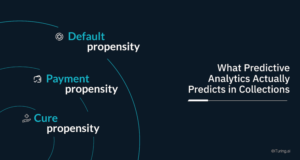
Default propensity is the probability that an account currently in good standing will become delinquent within the next 90 to 120 days. This is the early warning signal. It fires before a single payment is missed.

Payment propensity is the probability that an account already in delinquency will make a voluntary payment within a defined period. This is what helps collections teams prioritize which delinquent accounts deserve immediate attention and which ones can wait.

Cure propensity is the probability that a delinquent account will self-cure without any outreach at all. This prediction is equally important, and consistently underused. Contacting a borrower who was about to pay on their own wastes agent time, increases cost, and can push a cooperative borrower into a defensive posture.

Most banks running traditional collections operations rely only on the second type. They work accounts after default and guess at prioritization using blunt DPD (days past due) buckets. Predictive analytics software adds the other two layers, and that combination is where the real operational leverage lives.

The 120-Day Early Warning Window

The 120-day prediction horizon is not arbitrary. It reflects how financial stress actually develops in practice.

Borrowers rarely go from financial health to a missed payment overnight. The deterioration is gradual. It shows up in data weeks or months before the first payment is skipped. A borrower under growing financial stress will start drawing more heavily on their credit limit. Their transaction frequency drops. Mobile banking app logins become less frequent. They begin making only minimum payments on revolving credit. Spending shifts from discretionary categories toward essentials.

These are behavioural signals that also feed the churn prediction model layer running alongside default risk scoring. An account showing declining app engagement, reduced communication response rates, and minimum-only payment patterns is simultaneously a default risk candidate and a voluntary attrition risk. Separating those two signals within the 120-day window determines whether the right intervention is a hardship conversation or a retention offer, and deploying the wrong one erodes both recovery probability and the long-term customer relationship.

These signals will not appear on a credit report yet. They will not trigger any traditional risk alert. But they are observable in transaction data, account activity logs, and bureau inquiry patterns. And when combined and processed by a well-trained predictive model, they produce a risk score that is statistically reliable as far as 120 days ahead of the first missed payment.

FICO’s collections analytics framework captures this well: “Shifts in spending patterns, such as increased cash spending, higher credit limit utilization or a shift between different spending types, can signal financial distress before delinquency occurs.”

Getting to a 120-day window reliably requires the right data inputs, the right model architecture, and rigorous validation. Each of those deserves its own explanation.

The Input Signals That Actually Matter

Predictive analytics solutions for collections are only as good as the features they consume. The inputs divide into three categories, each adding a distinct layer of signal.

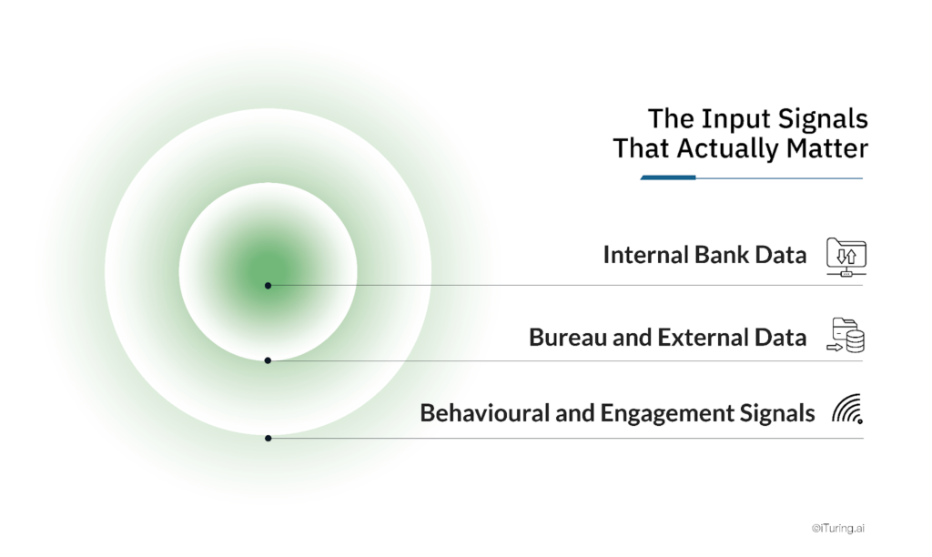
Internal Bank Data

This is the richest source. It includes payment history (amount, timing, and pattern across months), account age, product holdings across the bank, transaction frequency and volume, average balance trends over rolling 3, 6, and 12-month windows, and credit limit utilization ratios over time. Banks that can link current account data with mortgage, auto loan, and card data for the same customer have a meaningful modeling advantage. That cross-product view reveals stress patterns that a single-product view will miss entirely.

Bureau and External Data

Credit bureau tradelines reveal whether a borrower is showing stress across their entire credit portfolio, not just at your institution. Inquiry patterns, tradeline counts, public record activity, and changes in revolving balances across all lenders are all meaningful predictive inputs. The combination of internal account behavior plus cross-portfolio bureau signals substantially improves prediction accuracy at the 90-to-120-day horizon. A borrower who looks stable on your books but is accumulating stress across three other lenders is a risk your internal data alone will not surface.

Behavioural and Engagement Signals

This category is the most underused in traditional collections. It is also the input layer where ai predictive analytics delivers its most distinctive advantage over static scorecard approaches: processing the combination of mobile banking app login frequency, recent communication open rates, customer service contact history, and historical promise-to-pay adherence into forward-looking risk signals that no bureau pull can replicate. As research published in BFSI Eletsonline notes, AI systems can use “device and application usage, customer service interactions, and behavioral events such as changes in repayment behaviour” as predictive inputs alongside traditional financial data.

How the Models Actually Work

The most effective models for collections propensity prediction use gradient boosting algorithms, specifically XGBoost and LightGBM. These are ensemble learning methods that build a sequence of decision trees, each one correcting the residual errors of the one before it.

Gradient boosting models are well-suited to this task for two reasons. First, they handle mixed data types (numeric, categorical, temporal) without heavy preprocessing. Second, they capture non-linear relationships in the data that linear models like logistic regression consistently miss. In credit risk prediction tasks, gradient boosting achieves an AUC-ROC of 0.87 compared to 0.72 for logistic regression, and outperforms across precision, recall, and overall accuracy. That difference in discriminatory power translates directly to better account prioritization in collections.

The ai predictive analytics layer that runs on top of these models converts raw gradient boosting outputs into operationally usable signals: daily scores per account, threshold-based routing to the correct treatment band, and automated escalation when scores cross pre-defined risk levels. Feature engineering matters as much as the algorithm choice. The most predictive features for collections models include:

• Rolling windows: Payment velocity over 30, 60, and 90-day windows rather than point-in-time snapshots
• Velocity calculations: Rate of change in balance, utilization, and app login frequency
• Ratio features: Payment-to-minimum ratio, balance-to-limit ratio, and bureau balance versus bank balance
• Temporal patterns: Day-of-month payment behavior, seasonal patterns, and promotion response history

Models retrain on a monthly cadence. Financial behavior patterns shift with economic conditions, interest rate cycles, and labor market changes. A model trained on 2023 data without retraining will begin to decay in predictive accuracy across 2024 and 2025. Monthly retraining captures that concept drift before it degrades live model performance.

Validation: How Banks Know the Model Is Working

A propensity model without rigorous validation is a liability. The validation framework has three essential components.

Out-of-time testing is the gold standard approach. Train the model on 18 months of historical data. Validate it on the subsequent 6 months, where actual outcomes are already known. This tests whether the model would have correctly predicted what actually happened, not whether it simply memorized patterns in the training data.

Gini coefficient measures the model’s rank-ordering ability. A Gini of 0.40 or above indicates the model reliably separates high-risk accounts from low-risk ones. Below 0.35, the model’s discriminatory ability degrades to the point where its practical value in operations is limited. Gradient boosting models trained on well-prepared banking datasets routinely achieve Gini scores in the 0.50 to 0.70 range, a substantial improvement over traditional scorecards.

Back-testing closes the loop on the 120-day prediction claim specifically. The question is simple: did accounts that received a high-risk flag 120 days ago actually become delinquent? Back-testing this retrospectively across multiple cohorts gives the bank statistical confidence that the model’s predictions reflect real borrower dynamics, not artifacts of a particular data vintage or training period.

Precision-recall analysis determines where to set the intervention threshold. At what score does the bank trigger a preventive outreach? Setting the threshold too low generates too many false positives and overwhelms the preventive program with accounts that did not need intervention. Setting it too high misses accounts that did. The right threshold is a business decision informed by the cost of an intervention versus the expected cost of a missed prediction leading to default.

From Score to Strategy: Turning Predictions Into Recovery

The propensity score is the starting point. What the team does with it is what actually generates value.

A practical segmentation framework divides accounts into three bands based on their 120-day default propensity score.

High-risk accounts (top score band) receive proactive outreach within the prediction window. The contact strategy prioritizes soft, customer-centric messaging alongside hardship program options and payment plan offers. The objective is to address financial stress before a payment is ever missed. At this stage, the borrower is far more receptive to a supportive conversation than they will be after a default event.

Medium-risk accounts (middle band) receive enhanced monitoring and a lighter-touch digital communication sequence. SMS payment reminders, email notifications about upcoming due dates, and one targeted phone contact if no digital engagement occurs within a defined window.

Low-risk accounts (bottom band) continue through standard servicing. Predictive scoring confirms that collections resources do not need to be allocated here right now.

For cure propensity specifically, the churn prediction model output informs the routing decision before any contact is initiated. Accounts showing strong cure propensity signals alongside low churn risk receive at most a single low-cost digital reminder. Accounts showing cure propensity alongside elevated churn risk (declining engagement, reduced login frequency, deteriorating communication response rates) receive a retention-oriented contact rather than a standard collections sequence. Research and industry practice consistently shows that contacting a borrower who was going to pay anyway adds cost, consumes agent capacity, and can occasionally convert a cooperative borrower into an uncooperative one.

This is contact strategy optimization in practice. Which borrowers to reach out to, through which channel, at what point in the risk window, and whether to reach out at all are all decisions that flow from the propensity score. Get the scoring right, and every downstream decision in collections gets sharper.

How iTuring Approaches This

iTuring’s predictive analytics software generates 120-day early warnings with 83% prediction accuracy, drawing on a pre-built feature library of 25,000 features spanning payment behavior, transaction patterns, bureau signals, and engagement data. The platform delivers the full stack of ai predictive analytics for collections: default propensity, payment propensity, cure propensity, and churn prediction model outputs that route accounts to the correct intervention type before any contact decision is made.

Every account in the portfolio is scored daily. This is continuous assessment that updates as new transactions and behavioral signals arrive, not batch scoring on a monthly or weekly cycle. When an account crosses a risk threshold, the system flags it for preventive action immediately, not at the next reporting cycle.

Among predictive analytics solutions available to US banks, the platform deploys in four weeks with no IT overhead, integrates directly with core banking systems and existing collections CRM infrastructure, and includes built-in model validation reporting. That means compliance and risk teams have the documentation they need without commissioning a separate validation project.

For collections heads looking to make the shift from reactive to preventive, the starting point is understanding what your current portfolio’s 120-day risk picture actually looks like.

Regulatory Disclaimer
The information in this blog is provided for general informational purposes only and does not constitute legal, compliance, or regulatory advice. The deployment of predictive models in banking collections is subject to applicable regulatory guidance including the Federal Reserve’s SR 11-7 on model risk management, the Fair Debt Collection Practices Act (FDCPA), the Equal Credit Opportunity Act (ECOA), and relevant state-level regulations. Banks and financial institutions should consult qualified legal and compliance counsel before implementing AI-driven collections strategies. iTuring’s stated performance metrics are based on client implementations and may vary depending on data quality, portfolio composition, and deployment configuration.

Sources: Commercial Collection Agencies of America | FICO: Debt Collection Predictive Analytics | BFSI Eletsonline: AI-Driven Early Delinquency Prediction | IJCRT: Gradient Boosting Credit Risk Prediction | FinanceOps: Proactive Collections Strategy